Manipulating Chess-GPT's World Model

Manipulating Chess-GPT’s World Model

Note: This work has since been turned into a paper, but the average reader will probably prefer the blog post.

In my previous post I introduced Chess-GPT, a language model I trained to predict the next character in a game of chess given a PGN string (1.e4 e5 2.Nf3 …). Through the process of training to output the next character, it learns to compute the state of the chess board and to estimate the skill level of the players in the game given an arbitrary PGN string as input. I demonstrated this using linear probes, which are classifiers that take the model’s activations as input and predict the board state or player skill level as output. Chess-GPT also played chess well, with the best model playing at approximately 1500 Elo.

I presented evidence that the model learned to compute a world model in order to perform next character prediction, but I did not have the time to validate these representations by using them to intervene on the model’s activations. In other related work, the authors used the probes to edit Othello GPT’s internal activations, getting it to output legal moves under the “make believe” state of the board. I wanted to add rigor to my work and establish a causal link between the internal board state and skill representations and the model outputs. If there was a causal link, I should be able to increase and decrease the model’s skill level and edit its internal state of the board.

I had also done some investigation of Chess-GPT’s ability to play Chess in games very unlike those found in its training dataset (which consists of real games downloaded from Lichess). Specifically, I initialized the chess board with 20 random moves, and then had Chess-GPT play against Stockfish with this random initialization. Its performance plummeted. The larger 50 million parameter model’s win rate dropped from 70% to 17%. Did this mean that the models’ only learn superficial patterns of how to play Chess with no deeper understanding of the game? It turns out that this is not the case, and with one simple trick, we can restore a significant fraction of our models’ chess playing ability.

Next token predictors

When GPT-3 was released, some AI skeptics argued that GPT-3 learns surface statistics or correlations between words, with no understanding of the underlying world. Douglas Hofstadter (who no longer holds this position and is now worried about artificial super intelligence) argued that LLMs are “cluelessly clueless” because they produce nonsense when given trick questions. For example:

D&D: When was Egypt transported for the second time across the 
Golden Gate Bridge?

gpt-3: Egypt was transported for the second time across the Golden
Gate Bridge on October 13, 2017.

Gary Marcus and Ernest Davis, in their article “GPT-3, Bloviator: OpenAI’s language generator has no idea what it’s talking about”, also demonstrated that if you prompt GPT-3 with nonsense text, it will continue with nonsense text. Kevin Lacker gave GPT-3 a Turing Test, and found similar results.

Q: How do you sporgle a morgle?
A: You sporgle a morgle by using a sporgle.

Q: How many bonks are in a quoit?
A: There are three bonks in a quoit.

Q: How many rainbows does it take to jump from Hawaii to seventeen?
A: It takes two rainbows to jump from Hawaii to seventeen.

So what’s going on here? Does GPT-3 really have no ability to understand the world or express uncertainty? If we think about it further, GPT-3 is just trying to predict the next token as if the prompt is a section of a random piece of text on the internet. In this context, the text after to “How do you sporgle a morgle?” is much more likely to be “You sporgle a morgle by …” than “That question doesn’t make any sense!”. Base models without instruct tuning are finicky, and just because they answer nonsense with more nonsense doesn’t mean that they lack any understanding of the question. For example, Nick Cammarata showed GPT-3 can easily express uncertainty if we just prompt it to reply with “yo be real” to nonsense questions.

Of course, modern LLMs like ChatGPT or Claude are much more capable and have been trained on examples of desired behavior using RLHF or intruction tuning. Now, they correctly answer “I don’t know” to nonsense questions and express uncertainty about challenging questions. They don’t need to rely on prompts to elicit a desired behavior.

This suggests a possible explanation for Chess-GPT’s poor performance on randomly initialized games. If a game begins with 20 random moves, the players are probably not high skill players. Chess-GPT is also a base model, with no RLHF or instruct tuning to learn a desired behavior of playing strong chess. If Chess-GPT truly was a good next token predictor, it would predict legal, low skill moves in the case of a randomly initialized game.

To test this idea, I gave Chess-GPT randomly initialized games, and then recorded the Elo probe’s prediction for the White player. In normal games, the Elo probe would classify players as under 1550 Elo or above 2050 Elo, and it correctly classified 90.5% of players. In the case of randomly initialized games, the Elo probe classified 99.4% of players as low skill, indicating that the model was trying to predict the next character in a low skill game.

Skill Interventions

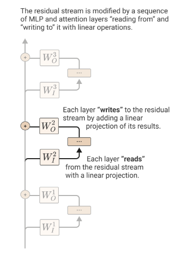
My linear probes are trained on the GPT’s residual stream. We can think of the residual stream as the intermediate state in a transformer, or the output of each layer before it is fed to the next layer. Each layer in the GPT reads from the residual stream, performs some calculation, and then adds the result back to the residual stream. In my case, the hidden dimension of Chess-GPT is 512, which means that the residual stream and every intermediate state is simply a 512 dimensional vector (or a list of 512 numbers). The following diagram is from Anthropic’s explanation of the transformer’s residual stream:

The linear probe for the Elo classification is a 512 x 2 matrix. We multiply the GPT’s 512 dimension activation vector with the Elo probe to produce a 2 dimensional vector¹, which contains raw predictions (also known as logits or scores) for low skill and high skill. By applying softmax, this 2 dimensional vector now contains probabilities that sum to 1. For example, an output of [0.2 0.8] means that the probe assigns an 80% probability to the player being a high skill player.

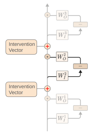
So, our Elo probe contains a 512 x 1 low skill vector and a 512 x 1 high skill vector. To create a skill intervention vector, we can subtract the low skill vector from the high skill vector. To encourage the model to play at a higher skill level, we can simply add this skill vector to the residual stream. Alternatively, we can add this vector to the layer’s final bias term to get an equivalent intervention at zero additional inference cost. We just flip the sign of the intervention to encourage the model to play at a lower skill level. To increase or decrease the magnitude of our intervention, we can multiply our intervention vector by a scaling factor. This intervention can be applied to an arbitrary number of layers, and is visualized here:

This intervention is extremely simple, and yet it works very well. I spent quite a bit of time experimenting with other more complicated interventions involving gradient descent and vector projection, and the simple addition baseline beat all other approaches that I tried. Of course, with machine learning, it’s hard to say that the addition technique is definitively better - there’s always the possibility that I just had to tweak one more detail and a more complicated approach would have been the best.

Here’s my intuition for why this works: The linear probe for low skill is trained to output a large positive value for low skill players and a large negative value for high skill players. These raw predictions (logits) are then converted to probabilities using softmax. For the probe to output a large positive value when multiplied with the model’s activations, the probe’s positive weights should align with positive activations, and negative weights with negative activations. Therefore, the low skill probe’s weights are oriented in a similar direction to the model’s internal representation of low skill play. Adding the skill vector (high skill minus low skill) to the activations encourages higher skill play by aligning the activations more closely with the high skill representation.

I also explored the technique of contrastive activations. In this technique, we collect the average GPT intermediate state activation per layer in 2,000 high skill games and 2,000 low skill games between turns 25 and 35. Once again, we subtract the average low skill activation from the average high skill activation to produce a skill vector. As with the probe-based intervention, this produces a 512 dimensional vector that we can add or subtract to the residual stream or final bias term. In practice, contrastive activations worked slightly better than probe derived interventions.

To test the effectiveness of this intervention, I had Chess-GPT play 30,000 games against Stockfish 16 level 0 across 6 configurations. The first three configurations had Chess-GPT play against Stockfish starting from the standard chess starting position. The last three had the board initialized with 20 randomly selected moves.

The resulting win rates are in this table:

Model	Board	No Intervention	Positive Intervention	Negative Intervention
50M Parameters	Standard	69.6%	72.3%	11.9%
25M Parameters	Standard	49.6%	54.8%	5.5%
50M Parameters	Randomly Initialized	16.7%	43.2%	5.9%
25M Parameters	Randomly Initialized	15.7%	31.3%	3.6%

In the standard board setting, adding the skill vector adds a minor increase in win rate, while subtracting it causes a substantial decrease. I believe the room for improvement in the standard setting is limited because the average skill level in the Lichess training dataset is 1,690 Elo, which is higher than Chess-GPT’s skill level.

However, the intervention works very well in the randomly initialized board. Here, the positive skill intervention improved the 25M parameter model’s win rate by 2x, and the 50M parameter model’s by 2.6x. The larger model’s more substantial improvement suggests that it may have more latent chess ability, and can perform better when it’s “trying” to win rather than emulate a low skilled player. This offers very strong evidence that, in the case of randomly initialized boards, the models are predicting the next character as if the players involved have a low skill level.

The intervention does only restore about half of the models’ performance. It’s difficult to say if this is because the models struggle to generalise to games that are very different from their training data, or if the models still have more latent ability that a better intervention could uncover. The addition intervention is very crude. It is adjusted via a scale parameter. If the scale is too low, it doesn’t make a difference, and if it’s too high, the model outputs random characters rather than valid chess moves. With the current primitive state of ML science and interpretability, it’s difficult to say which is the case.

Board State Interventions

In my previous post, I also found that Chess-GPT learns to compute the state of the chess board from a PGN string input. To validate these board state representations, I also wanted to perform interventions to edit Chess-GPT’s beliefs about the current board state. If my intervention was successful, Chess-GPT should output moves that are legal under the new, modified state of the chess board.

When modifying the chess board, we need to make sure that our change is strategically relevant to the current state of the board. If we modify a random piece, most of the existing legal moves will remain legal, and the randomly changed piece will probably not be selected by Chess-GPT if it isn’t in a strategically important position. My strategy was the following:

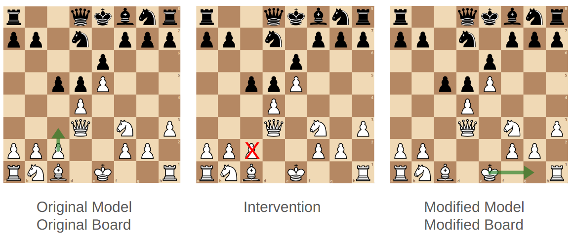
First, I sampled Chess-GPT’s most likely move by giving it a PGN string and sampling the maximum likelihood character at every prediction. Then, I determine the piece that was moved and its source square. In this case, it’s White pawn from C2. This gives us a strategically relevant piece at a current board state.

Now, I delete the piece from both the model’s internal representation and the original board to create a modified model and modified board. In this case, I delete the White pawn from C2 off the chess board. Then, I select the 512 dimensional White pawn row from the linear probe for square C2. I then subtract the C2 white pawn vector from the model’s residual stream, effectively “erasing” the model’s memory of the pawn’s presence on C2.

Then, I sample five probabilistic moves from both the original and modified model at temperature 1.0. The original model’s moves provide a baseline legal move rate without any intervention. If my intervention was successful, all 5 moves from the modified model would be legal under the new state of the chess board.

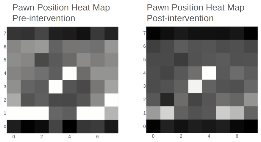
In the following diagram, I display the white pawn heat map before intervention (where Chess-GPT chose to move the white pawn from c2-c3) and after intervention, when the c2 pawn was erased from Chess-GPT’s internal activations. We can use linear probes to create visual heatmaps of Chess-GPT’s internal board state. Each linear probe outputs a probability that a particular piece (such as white pawn) is present on a particular square. We can use these outputs to construct a heat map for any piece type.

As we can see, post intervention the c2 pawn is indeed missing. However, the other white pawn locations are much less distinct, indicating that the intervention is fairly crude, even if successful.

I perform this intervention in 5,000 test cases. As the table below shows, my approach performs significantly better than the baseline of 41% legal moves. However, even in the best case the legal move rate is only 92%. Once again, it’s difficult to say if this is because of my primitive intervention strategy or if the model has a poor internal representation of the state of the board.

Model	Intervention Status	Original Board	Modified Board
50M Parameters	With Intervention	85.4%	92.0%
25M Parameters	With Intervention	81.8%	90.4%
50M Parameters	No Intervention	99.9%	40.5%
25M Parameters	No Intervention	99.8%	41.0%

Implications

These experiments significantly strength the findings of my previous blog post, suggesting that Chess-GPT learns a deeper understanding of chess strategy and rules, rather than simply memorizing patterns. Chess-GPT is orders of magnitude smaller than any current LLM and can be trained in 2 days on 2 RTX 3090 GPUs, yet it still manages to learn to estimate latent variables such as player skill. In addition, we see that bigger models learn to better compute board state and player skill.

This adds further evidence that language models can develop a world model through the process of next token prediction and self supervised learning. Whatever is going on inside these models is much more sophisticated than surface-level stastics. The success of the interventions adds further evidence that it is possible to directly influence model behavior in predictable ways using simple tools.

However, the fact that these interventions are only partially successful highlights the limitations of our current understanding of machine learning models. The current state of interpretability in machine learning is still fairly primitive and comparable to the early, pre-microscope days in biology. More research is needed to develop more precise and reliable methods of understanding language models. Fortunately, there are exciting new innovations such as Sparse Autoencoders which have shown promising results.

All code, models, and datasets can be found at:

https://github.com/adamkarvonen/chess_llm_interpretability

If interested in discussion or collaboration, feel free to contact me via email.

I am currently open to job opportunities. If you found this post interesting and think I could be a good fit for your team, feel free to reach out via email or LinkedIn.

There is also this Twitter thead for public discussion purposes.

Appendix

Other Interventions

When performing probe based skill interventions, I found that it was possible to improve Chess-GPT’s ability by adding the high skill vector, subtracting the low skill vector, or both adding the high skill vector and subtracting the low skill vector. However, I got the best results from performing both interventions. In contrast, with board state interventions, I found that I got the best results by only subtracting the moved piece vector. Adding the blank square vector lowered the success rate of the intervention.

One very important hyperparameter in these interventions is the scale parameter, which is multiplied by the intervention vector. If it was too low, the modified model would make the same illegal moves as the original model. If it was too high, the modified model would output random characters. To estimate the upper bound of the success rate for board state interventions, I explored varying the scale of intervention across a range of values for each move to identify a scale that resulted in the model generating legal moves. I found a scale that resulted in the model outputting legal moves approximately 98\% of the time.

I looked at a couple options to dynamically set the scale parameter. The first was vector projection from the Representation Engineering paper. The second was to use some algebra to set the scale parameter to target a specific output logit value for the linear probe. In this case, the target value was another parameter to sweep, and -10 seemed to work well.

I explored a range of other interventions to try and increase the success of my board state interventions. Kenneth Li had originally used gradient descent with his non-linear probes. The probes are trained using cross-entropy loss, which is basically trying to maximize the probability output for the ground truth label. To perform an intervention with gradient descent, our loss is once again the cross entropy loss between the probe output probability and the desired board state (in this case, a blank square). Instead of optimizing the probe weights to minimze loss, we optimize the model activations being input to the linear probe.

In all of these cases, the simplest approach of just subtracting the piece vector from the residual stream worked the best. As is often the case, reality was not kind to my clever ideas and the simplest approach won. Out of all alternative approaches, the target logit value approach worked the best, but was still around 1-2% worse than the subtraction approach.

The best positive intervention win rates in the random board state using probe derived interventions were 42.2% for the 50M parameter model, and 24.7% for the 25M parameter model.

1. In matrix multiplication, multiplying a 1 x 512 matrix (or vector) by a 512 x 2 matrix produces a 1 x 2 matrix (or vector) as the result. The first row of 512 numbers, when multipled via dot product with the 512 dimensional activation, produces a score for “low skill player”. The second row of 512 numbers produces a score for “high skill player” when multipled with the activation. ↩