An Intuitive Explanation of Sparse Autoencoders for LLM Interpretability

Sparse Autoencoders (SAEs) have recently become popular for interpretability of machine learning models (although sparse dictionary learning has been around since 1997). Machine learning models and LLMs are becoming more powerful and useful, but they are still black boxes, and we don’t understand how they do the things that they are capable of. It seems like it would be useful if we could understand how they work.

Using SAEs, we can begin to break down a model’s computation into understandable components. There are several existing explanations of SAEs, and I wanted to create a brief writeup from a different angle with an intuitive explanation of how they work.

Challenges with interpretability

The most natural component of a neural network is individual neurons. Unfortunately, individual neurons do not conveniently correspond to single concepts. An example neuron in a language model corresponded to academic citations, English dialogue, HTTP requests, and Korean text. This is a concept called superposition, where concepts in a neural network are represented by combinations of neurons.

This may occur because many variables existing in the world are naturally sparse. For example, the birthplace of an individual celebrity may come up in less than one in a billion training tokens, yet modern LLMs will learn this fact and an extraordinary amount of other facts about the world. Superposition may emerge because there are more individual facts and concepts in the training data than neurons in the model.

Sparse autoencoders have recently gained popularity as a technique to break neural networks down into understandable components. SAEs were inspired by the sparse coding hypothesis in neuroscience. Interestingly, SAEs are one of the most promising tools to interpret artificial neural networks. SAEs are similar to a standard autoencoder.

A regular autoencoder is a neural network designed to compress and then reconstruct its input data. For example, it may receive a 100 dimensional vector (a list of 100 numbers) as input, feed this input through an encoder layer to compress the input to a 50 dimensional vector, and then feed the compressed encoded representation through the decoder to produce a 100 dimensional output vector. The reconstruction is typically imperfect because the compression makes the task challenging.

Diagram of a standard autoencoder with a 1x4 input vector, 1x2 intermediate state vector, and 1x4 output vector. The cell colors indicate activation value. The output is an imperfect reconstruction of the input.

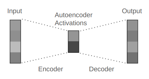
Sparse Autoencoder Explanation

How Sparse Autoencoders Work

A sparse autoencoder transforms the input vector into an intermediate vector, which can be of higher, equal, or lower dimension compared to the input. When applied to LLMs, the intermediate vector’s dimension is typically larger than the input’s. In that case, without additional constraints the task is trivial, and the SAE could use the identity matrix to perfectly reconstruct the input without telling us anything interesting. As an additional constraint, we add a sparsity penalty to the training loss, which incentivizes the SAE to create a sparse intermediate vector. For example, we could expand the 100 dimensional input into a 200 dimensional encoded representation vector, and we could train the SAE to only have ~20 nonzero elements in the encoded representation.

Diagram of a sparse autoencoder. Note that the intermediate activations are sparse, with only 2 nonzero values.

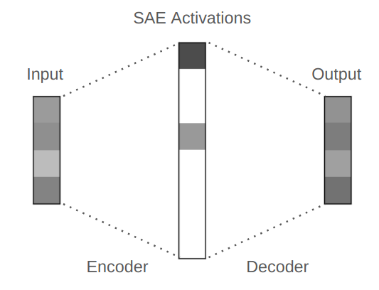
We apply SAEs to the intermediate activations within neural networks, which can be composed of many layers. During a forward pass, there are intermediate activations within and between each layer. For example, GPT-3 has 96 layers. During the forward pass, there is a 12,288 dimensional vector (a list of 12,288 numbers) for each token in the input that is passed from layer to layer. This vector accumulates all of the information that the model uses to predict the next token as it is processed by each layer, but it is opaque and it’s difficult to understand what information is contained within.

We can use SAEs to understand this intermediate activation. An SAE is basically a matrix -> ReLU activation -> matrix¹². As an example, if our GPT-3 SAE has an expansion factor of 4, the input activation is 12,288 dimensional and the SAE’s encoded representation is 49,512 dimensional (12,288 x 4). The first matrix is the encoder matrix of shape (12,288, 49,512) and the second matrix is the decoder matrix of shape (49,512, 12,288). By multiplying the GPT’s activation with the encoder and applying the ReLU, we produce a 49,512 dimensional SAE encoded representation that is sparse, as the SAE’s loss function incentivizes sparsity. Typically, we aim to have less than 100 numbers in the SAE’s representation be nonzero. By multiplying the SAE’s representation with the decoder, we produce a 12,288 dimensional reconstructed model activation. This reconstruction doesn’t perfectly match the original GPT activation because our sparsity constraint makes the task difficult.

We train individual SAEs on only one location in the model. For example, we could train a single SAE on intermediate activations between layers 26 and 27. To analyze the information contained in the outputs of all 96 layers in GPT-3, we would train 96 separate SAEs - one for each layer’s output. If we also wanted to analyze various intermediate activations within each layer, this would require hundreds of SAEs. Our training data for these SAEs comes from feeding a diverse range of text through the GPT model and collecting the intermediate activations at each chosen location.

I’ve included a reference SAE Pytorch implementation. The variables have shape annotations following Noam Shazeer’s tip. Note that various SAE implementations will often have various bias terms, normalization schemes, or initialization schemes to squeeze out additional performance. One of the most common additions is some sort of constraint on decoder vector norms. For more details, refer to various implementations such as OpenAI’s, SAELens, or dictionary_learning.

import torch
import torch.nn as nn

# D = d_model, F = dictionary_size
# e.g. if d_model = 12288 and dictionary_size = 49152
# then model_activations_D.shape = (12288,) and encoder_DF.weight.shape = (12288, 49152)

class SparseAutoEncoder(nn.Module):
    """
    A one-layer autoencoder.
    """
    def __init__(self, activation_dim: int, dict_size: int):
        super().__init__()
        self.activation_dim = activation_dim
        self.dict_size = dict_size

        self.encoder_DF = nn.Linear(activation_dim, dict_size, bias=True)
        self.decoder_FD = nn.Linear(dict_size, activation_dim, bias=True)

    def encode(self, model_activations_D: torch.Tensor) -> torch.Tensor:
        return nn.ReLU()(self.encoder_DF(model_activations_D))
    
    def decode(self, encoded_representation_F: torch.Tensor) -> torch.Tensor:
        return self.decoder_FD(encoded_representation_F)
    
    def forward_pass(self, model_activations_D: torch.Tensor) -> tuple[torch.Tensor, torch.Tensor]:
        encoded_representation_F = self.encode(model_activations_D)
        reconstructed_model_activations_D = self.decode(encoded_representation_F)
        return reconstructed_model_activations_D, encoded_representation_F

The loss function for a standard autoencoder is based on the accuracy of input reconstruction. To introduce sparsity, early SAE implementations added a sparsity penalty to the SAE’s loss function. This most common form of this penalty is calculated by taking the L1 loss of the SAE’s encoded representation (not the SAE weights) and multiplying it by an L1 coefficient. The L1 coefficient is a crucial hyperparameter in SAE training, as it determines the trade-off between achieving sparsity and maintaining reconstruction accuracy.

Note that we aren’t optimizing for interpretability. Instead, we obtain interpretable SAE features as a side effect of optimizing for sparsity and reconstruction.

Here is a reference loss function.

# B = batch size, D = d_model, F = dictionary_size

def calculate_loss(autoencoder: SparseAutoEncoder, model_activations_BD: torch.Tensor, l1_coeffient: float) -> torch.Tensor:
    reconstructed_model_activations_BD, encoded_representation_BF = autoencoder.forward_pass(model_activations_BD)
    reconstruction_error_BD = (reconstructed_model_activations_BD - model_activations_BD).pow(2)
    reconstruction_error_B = einops.reduce(reconstruction_error_BD, 'B D -> B', 'sum')
    l2_loss = reconstruction_error_B.mean()

    l1_loss = l1_coefficient * encoded_representation_BF.sum()
    loss = l2_loss + l1_loss
    return loss

UPDATE 11/29/2024: I think the Vanilla ReLU SAE is fairly outdated and should not be used except as a baseline. My preferred SAE is the TopK SAE, as it significantly improves on the sparsity / reconstruction accuracy trade-off, the desired sparsity can be directly set without tuning a sparsity penalty, and it has good training stability. The TopK SAE is very similar to the ReLU SAE. Instead of a ReLU and a sparsity penalty, you simply retain the top k activation values and zero out the rest. In this case, the k hyperparameter directly sets the desired sparsity. An example TopK implementation can be seen here. Other strong alternative approaches are the BatchTopK and JumpReLU SAEs.

A single Sparse Autoencoder forward pass. We begin with a 1x4 model vector. We multiply it with a 4x8 encoder matrix to produce a 1x8 encoded vector, then apply the ReLU to zero out negative values. The encoded vector is sparse. We multiply it with a 8x4 decoder matrix to produce a 1x4 imperfectly reconstructed model activation.

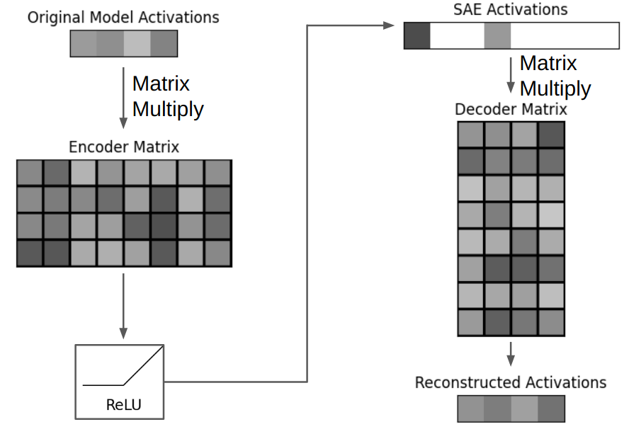
A Hypothetical SAE Feature Walkthrough

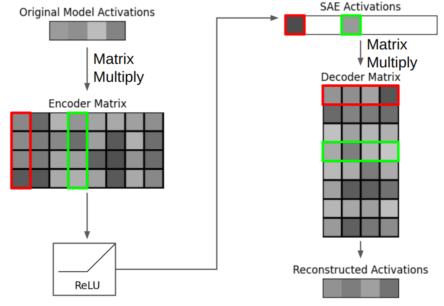
Hopefully, each active number in the SAE’s representation corresponds to some understandable component. As a hypothetical example, assume that the 12,288 dimensional vector [1.5, 0.2, -1.2, ...] means “Golden Retriever” to GPT-3. The SAE decoder is a matrix of shape (49,512, 12,288), but we can also think of it as a collection of 49,512 vectors, with each vector being of shape (1, 12,288). If the SAE decoder vector 317 has learned the same “Golden Retriever” concept as GPT-3, then the decoder vector would approximately equal [1.5, 0.2, -1.2, ...]. Whenever element 317 of the SAE’s activation is nonzero, a vector corresponding to “Golden Retriever” (and scaled by element 317’s magnitude) will be added to the reconstructed activation. In the jargon of mechanistic interpretability, this can be succinctly described as “decoder vectors correspond to linear representations of features in residual stream space”.

This makes intuitive sense when we consider the mathematics of vector-matrix multiplication. Multiplying a vector with a matrix is essentially a weighted sum of the matrix’s rows (or columns, depending on the multiplication order), where the weights are the elements of the vector. In our case, the SAE’s sparse encoded representation serves as these weights, selectively activating and scaling the relevant decoder vectors (matrix rows) to reconstruct the original activation.

We can also say that our SAE with a 49,512 dimensional encoded representation has 49,512 features. A feature is composed of the corresponding encoder and decoder vectors. The role of the encoder vector is to detect the model’s internal concept while minimizing interference with other concepts, while the decoder vector’s role is to represent the “true” feature direction. Empirically, we find that encoder and decoder vectors for each feature are different, with a median cosine similarity of 0.5. In the below diagram, the three red boxes correspond to a single feature.

The three red boxes correspond to SAE feature 1, and the green boxes correspond to feature 4. Per feature, there is a 1x4 encoder vector, 1x1 feature activation, and 1x4 decoder vector. The reconstructed activation is only constructed from the decoder vectors from SAE features 1 and 4. If red represents the color red, and green represents a sphere, then the model could be representing a red sphere.

How do we know what our hypothetical feature 317 represents? The current practice is to just look at the inputs that maximally activate the feature and give a gut reaction on their interpretability. The inputs each feature activates on are frequently interpretable. For example, Anthropic trained SAEs on Claude Sonnet and found separate SAE features that activate on text and images related to the Golden Gate Bridge, neuroscience, and popular tourist attractions. Other features activate on concepts that aren’t immediately obvious, such as a feature from a SAE trained on Pythia that activates “on the final token of relative clauses or prepositional phrases which modify a sentence’s subject”.

Because the SAE decoder vectors match the shape of the LLMs intermediate activations, we can perform causal interventions by simply adding decoder vectors to model activations. We can scale the strength of the intervention by multiplying the decoder vector with a scaling factor. When Anthropic researchers added the Golden Gate Bridge SAE decoder vector to Claude’s activations, Claude was compelled to mention the Golden Gate Bridge in every response.

Here is a reference implementation of a causal intervention using our hypothetical feature 317³. This very simple intervention would compel our GPT-3 model to mention Golden Retrievers in every response, similar to Golden Gate Bridge Claude.

def perform_intervention(model_activations_D: torch.Tensor, decoder_FD: torch.Tensor, scale: float) -> torch.Tensor:
    intervention_vector_D = decoder_FD[317, :]
    scaled_intervention_vector_D = intervention_vector_D * scale
    modified_model_activations_D = model_activations_D + scaled_intervention_vector_D
    return modified_model_activations_D

Challenges with Sparse Autoencoder Evaluations

One of the main challenges with using SAEs is in evaluation. We are training sparse autoencoders to interpret language models, but we don’t have a measurable underlying ground truth in natural language. Currently, our evaluations are subjective, and basically correspond to “we looked at activating inputs for a range of features and gave a gut reaction on interpretability of the features”. This is a major limitation in the field of interpretability.

Researchers have found common proxy metrics that seem to correspond to feature interpretability. The most commonly used are L0 and Loss Recovered. L0 is the average number of nonzero elements in the SAE’s encoded intermediate representation. Loss Recovered is where we replace the GPT’s original activation with our reconstructed activation and measure the additional loss from the imperfect reconstruction. There is typically a trade-off between these two metrics, as SAEs may choose a solution that decreases reconstruction accuracy to increase sparsity.

A common comparison of SAEs involves graphing these two variables and examining the tradeoff⁴. Many new SAE approaches, such as Deepmind’s Gated SAE and OpenAI’s TopK SAE, modify the sparsity penalty to improve on this tradeoff. The following graph is from Google Deepmind’s Gated SAE paper. The red line for Gated SAEs is closer to the top left of the graph, meaning that it performs better on this tradeoff.

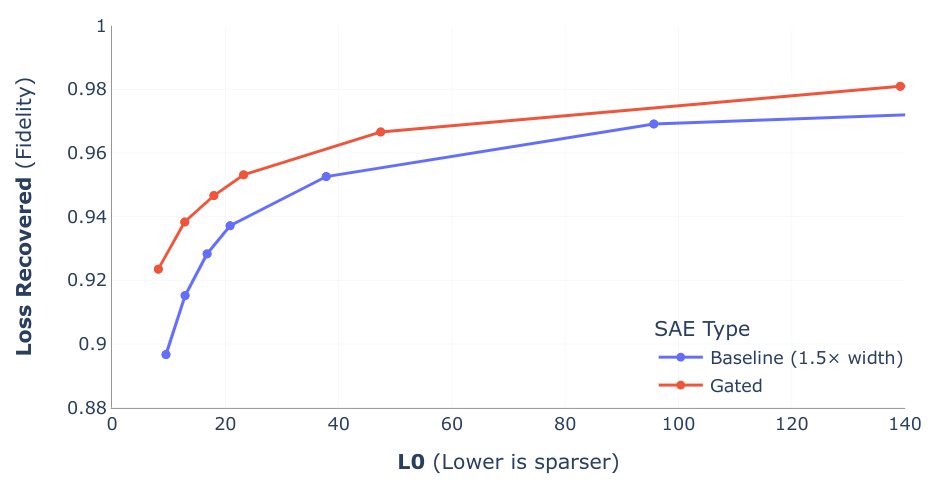
There’s several layers to difficulties with measurements in SAEs. Our proxy metrics are L0 and Loss Recovered. However, we don’t use these when training as L0 isn’t differentiable and calculating Loss Recovered during SAE training is computationally expensive⁵. Instead, our training loss is determined by an L1 penalty and the accuracy of reconstructing the internal activation, rather than its effect on downstream loss.

Our training loss function doesn’t directly correspond to our proxy metrics, and our proxy metrics are only proxies for our subjective evaluations of feature interpretability. There’s an additional layer of mismatch, as our subjective interpretability evaluations are proxies for our true goal of “how does this model work”. There’s a possibility that some important concepts within LLMs are not easily interpretable, and we could ignore these by blindly optimizing interpretability.

For a more detailed discussion of SAE evaluation methods and an evaluation approach using board game model SAEs, refer to my blog post on Evaluating Sparse Autoencoders with Board Game Models.

Conclusion

The field of interpretability has a long way to go, but SAEs represent real progress. They enable interesting new applications, such as an unsupervised method to find steering vectors like the “Golden Gate Bridge” steering vector. SAEs have also made it easier to find circuits in language models, which can potentially be used to remove unwanted biases from the internals of the model.

The fact that SAEs find interpretable features, even though their objective is merely to identify patterns in activations, suggests that they are uncovering something meaningful. This is also evidence that LLMs are learning something meaningful, rather than just memorizing surface-level statistics.

They also represent an early milestone that companies such as Anthropic have aimed for, which is “An MRI for ML models”. They currently do not offer perfect understanding, but they may be useful to detect unwanted behavior. The challenges with SAEs and SAE evaluations are not insurmountable and are the subject of much ongoing research.

For further study of Sparse Autoencoders, I recommend Callum McDougal’s Colab notebook.

Acknowledgements: I am grateful to Justis Mills, Can Rager, Oscar Obeso, and Slava Chalnev for their valuable feedback on this post.

1. The ReLU activation function is simply y = max(0, x). That is, any negative input is set to 0. ↩

2. There are typically also bias terms at various points, including the encoder and decoder layers. ↩

3. Note that this function would intervene on a single layer and that the SAE should have been trained on the same location as the model activations. For example, if the intervention was performed between layers 6 and 7 then the SAE should have been trained on the model activations between layers 6 and 7. Interventions can also be performed simultaneously on multiple layers. ↩

4. It’s worth noting that this is only a proxy and that improving this tradeoff may not always be better. As mentioned in the recent OpenAI TopK SAE paper, an infinitely wide SAE could achieve a perfect Loss Recovered with an L0 of 1 while being totally uninteresting. ↩

5. Apollo Research recently released a paper that used a loss function that aimed to produce the same output distribution, rather than reconstruct a single layer’s activation. It works better but is also more computationally expensive. ↩