Evaluating Sparse Autoencoders with Board Games

This blog post discusses a collaborative research paper on sparse autoencoders (SAEs), specifically focusing on SAE evaluations and a new training method we call p-annealing. As the first author, I primarily contributed to the evaluation portion of our work. The views expressed here are my own and do not necessarily reflect the perspectives of my co-authors. You can access our full paper here.

Key Results

In our research on evaluating Sparse Autoencoders (SAEs) using board games, we had several key findings:

• We developed two new metrics for evaluating Sparse Autoencoders (SAEs) in the context of board games: board reconstruction and coverage.

• These metrics can measure progress between SAE training approaches that is invisible on existing metrics.

• These metrics allow for meaningful comparisons between different SAE architectures and training methods, potentially informing SAE design for more complex domains like language models.

• We introduce p-annealing, a new SAE training method that improves over prior methods on both existing metrics and our new metrics.

• SAEs trained on ChessGPT and OthelloGPT can capture a substantial fraction of the model’s board state, with F1 scores of 0.85 and 0.95 respectively for board reconstruction.

• However, SAEs do not match the performance of linear probes, suggesting they may not capture all of the model’s board state information or “world model”.

Challenges with SAE Evaluations

For an explanation of sparse autoencoders, refer to my Introduction to SAEs.

Sparse Autoencoders (SAEs) have recently become popular for interpretability of machine learning models. Using SAEs, we can begin to break down a model’s computation into understandable components. As a result, there have been a flurry of new SAE architectures and loss functions, such as the BatchTopK SAE, Google Deepmind’s Gated SAE and JumpReLU SAE, our p-annealing, and OpenAI’s TopK SAE.

Unfortunately, we don’t have reliable metrics that we can use to compare the new approaches. The main metric currently used is “we looked at activating inputs for a range of features and gave a gut reaction on interpretability of the features”. This is a major limitation for the field.

In machine learning, it’s ideal to have an objective evaluation of your model, such as accuracy on the MNIST benchmark. With an objective evaluation, you can just twiddle all the knobs of architectures, hyperparameters, loss functions, etc, and see which knobs make the number go up. When measuring the interpretability of SAEs trained on language models, there is no underlying ground truth that we know how to measure. We do have some proxy metrics, such as L0 (a measure of SAE sparsity) and loss recovered (a measure of SAE reconstruction fidelity), that seem to have some correlation with interpretability. However, they are only proxies for the thing we care about and can sometimes be inversely correlated with interpretability.

An example of subjective interpretability from Anthropic's Scaling Monosemanticity. In this case, it looks like the feature activates on phrases related to transit infrastructure.

As a result, we primarily use noisy, time-consuming subjective evaluations. When crowd workers subjectively evaluated the interpretability of Deepmind’s Gated SAE, the results were not statistically significant. It’s hard to say whether this is due to the inherent noisiness of our evaluation methods or if it points to some limitation of the Gated SAE architecture itself. Interpretability also isn’t all we care about, as important parts of model cognition may not be easily interpretable.

There have been some recent examples of different natural language evaluations. In this case, across various SAEs Anthropic examined how many elements from the periodic table had corresponding SAE features. While interesting, there are obvious limitations. Periodic table elements are a very limited subset of natural language, and it’s challenging to robustly measure natural language concepts. String matching has trouble differentiating different uses of the word “lead”, which can be an element or a verb. It’s even more difficult to measure abstract concepts not closely tied to a single word.

While we don’t know how to measure the underlying ground truth of natural language, board games have a measurable ground truth and are still reasonably complex. We used Chess and Othello as testbeds for SAEs with two questions in mind.

1. How can we measure and compare different SAEs?
2. What fraction of the model’s “world model” or board state do the SAEs capture?

All code, datasets, and models for these evaluations have been open sourced at github.com/adamkarvonen/SAE_BoardGameEval.

Sparse Autoencoder Coverage Metric

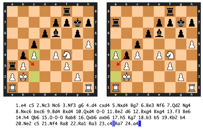
Our first metric is called coverage. We created measurable units of the board, which we called Board State Properties (BSPs). We defined ~1000 BSPs, including low-level details like “Is one of my knights on F3?” and high-level concepts like “Is there a pinned piece on the board?”. Because these are measurable with code, we could automatically find thousands of interpretable features without any manual interpretability. For example, we found the below “en passant capture available” feature. It’s very impressive that SAEs, which are unsupervised, manage to find these interesting concepts.

An example "en passant capture available" feature. Notice that it only fires twice on space characters in the PGN string, both times when the current player had an en passant capture available.

To calculate the coverage metric, we first find best classifying feature for each possible BSP as measured by the F1 score. We then average the F1 scores of these best features, as shown below.

A demonstration of calculating coverage for all low-level Chess BSPs.

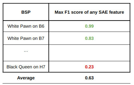
If the SAE has features that directly correspond to individual Chess or Othello concepts, the average best F1 score will be high. On the other hand, if the SAE mainly captures combinations of concepts, the average best F1 score will be lower, as no single feature will be a good classifier for individual square states. Thus, the coverage metric serves as a proxy for monosemanticity or the quality of SAE features. Note that without a good scientific understanding of what’s happening inside transformer models, it isn’t clear what the maximum coverage score should be. It’s possible that an SAE faithfully reconstructing model representations should achieve a coverage significantly below 1.0.

The following table contains the best coverage scores obtained at layer 6 by any SAE. As baselines, we test the exact same approach on layer 6 MLP activations (note that this comparison, with no SAE, was done after paper submission), and on SAEs trained on versions of ChessGPT and OthelloGPT with randomly initialized weights.

Approach	ChessGPT	OthelloGPT
SAE RandomGPT	0.11	0.27
MLP Activations	0.26	0.53
SAE TrainedGPT	0.45	0.52

SAEs on the trained models substantially outperform the random model baseline, indicating that they capture meaningful information. Surprisingly, MLP activations on OthelloGPT perform quite well, suggesting that some board state information is directly encoded in MLP neuron activations.

Sparse Autoencoder Board Reconstruction Metric

The coverage metric provides insight into the quality of SAE features, but it doesn’t consider the breadth of knowledge captured by the SAE. When we look at large language models predicting the next token in text, it’s often unclear what the complete underlying world state is. It’s challenging to measure exactly what the model ‘knows’ at each step of the prediction process. However, in games like Chess and Othello, we have a clear, measurable world state at every token. With this in mind, we developed the Board Reconstruction Metric. The key question we’re asking is: Can we completely reconstruct the board state from model activations using a Sparse Autoencoder¹?

An important question is which assumptions we make about what SAE features should mean. There had been prior work on applying SAEs to OthelloGPT. In Othello, there are 64 squares and 3 possible states for each square (Black, White, and Empty), or 192 (64 x 3) possible square states. The author had looked for individual features that were accurate classifiers with both high precision and recall for an individual square state. Using this approach, they found classifiers for only 33 of the square states.

We instead looked for features that had at least 95% precision (an arbitrary threshold) for square states, without necessarily having high recall. That is, if the feature was active, the square state is present. This was motivated in part by studies on chess players showing that chess experts excel at remembering realistic board configurations, but not random piece placements. This suggests experts (and potentially AI models) encode board states as meaningful patterns rather than individual square occupancies.

To identify high-precision features, we analyzed how each feature’s activation corresponds to board states. Our approach was as follows:

1. We determined each feature’s maximum activation value across 256,000 tokens.
2. We set 10 threshold values per feature, from 0% to 90% of its maximum activation.
3. For each threshold, we identified all high precision features.

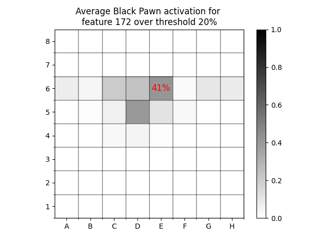
As an example, let’s look at the probability that a black pawn is on every square for SAE feature 172 at threshold 20%²³. This example analysis was performed on a set of 1,000 “train” games. As we can see, the feature is not high precision for any square, and there is a broad distribution over squares.

On the other hand, there is a 98% chance that a White Knight is on F3 any time the feature is active at all.

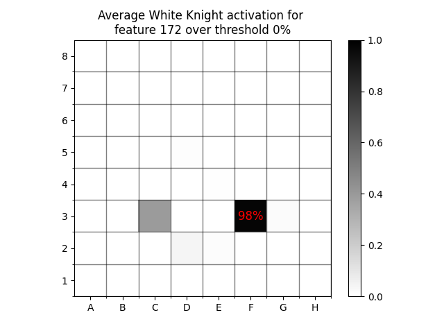
A common finding is that SAE activations become more interpretable at higher values. When we increase the threshold to 20%, there is a 100% chance that a White Knight is on F3.

This increasing certainty happens at different rates for different piece types. For example, at threshold 0% there is a 79% chance that there’s a black bishop on G4.

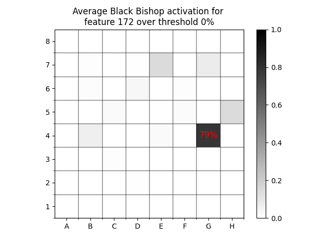
If we increase the threshold to 50%, then the likelihood of a black bishop being on G4 increases to 98%, meaning that feature 172 is high precision for two separate pieces at a threshold of 50%.

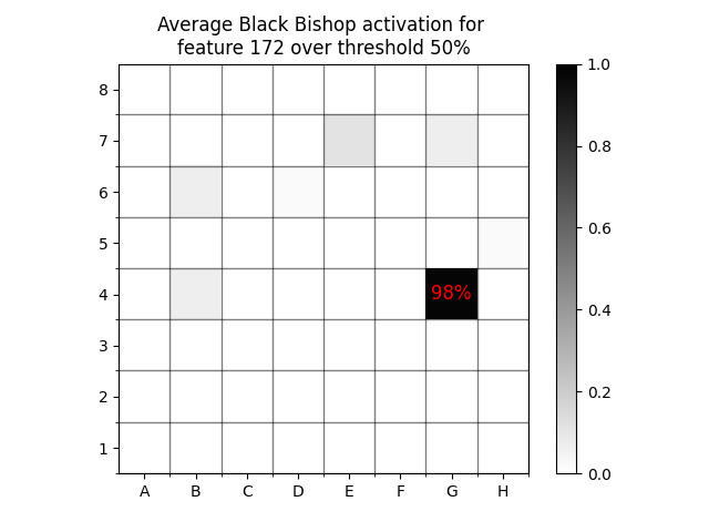
What can we do with this information? We can count the number of High Precision Classifier (HPC) features that classify a square with over 95% precision (an arbitrary precision threshold) at every activation threshold, but that doesn’t tell us how much of the model’s board state information is captured. As a proxy for recall, we can use our SAE’s HPC features to reconstruct the chess board on an unseen set of “test” games. We calculate the F1 score at every threshold value, and report the maximum score obtained. The best threshold is typically 0%, 10%, or 20%.

A demonstration of calculating board reconstruction for all low-level Chess BSPs.

In our paper, we call this metric board reconstruction. The following table contains the best board reconstruction score obtained across all SAEs trained on layer 6 of ChessGPT and OthelloGPT, in addition to previously mentioned baselines. We also compare to linear probes trained on layer 6.

Approach	ChessGPT	OthelloGPT
SAE RandomGPT	0.01	0.08
MLP Activations	0.56	0.82
SAE TrainedGPT	0.85	0.95
Linear Probe	0.98	0.99

SAEs on the trained model substantially outperform SAEs trained on the randomly initialized models, indicating that this is capturing genuine model board state information, but do not meet the performance of linear probes. This possibly means that current SAE techniques do not capture all of the model’s board state. The approach works surprisingly well on MLP activations, although SAEs perform better.

We also apply this approach to reconstructing high-level chess board state features. It works well for some, such as if an en passant capture is available (F1 score 0.92), and worse for others, such as if a pinned piece is on the board (F1 score 0.20).

P-Annealing: A New SAE Training Approach

We developed our metrics with the purpose of measuring progress in SAE training methods. These metrics allowed us to evaluate a new SAE training method we propose called p-annealing, which aims to address some fundamental challenges in training sparse autoencoders.

Ideally, we want our SAEs to be sparse as measured by L0 (the number of non-zero elements), but L0 is not differentiable and thus can’t be directly optimized. Traditionally, we instead train SAEs with the L1 loss as a differentiable proxy for sparsity. However, this approach leads to issues such as feature shrinkage.

P-annealing addresses this issue by leveraging nonconvex L_p^p minimization, where p<1. “Nonconvex” here means the optimization landscape may contain multiple local minima or saddle points, meaning that simple gradient optimization may get stuck in non-optimal solutions. We start training using convex L1 minimization (p=1), which is easier to optimize without getting stuck in local optima. We gradually decrease p during training, resulting in closer approximations of the true sparsity measure, L0, as p approaches 0.

In our evaluations using the board reconstruction and coverage metrics, we found that p-annealing led to significant improvements in SAE performance, which we’ll discuss in detail in the following section.

Comparing SAEs

In our evaluation, we compared four SAE types using our metrics: the standard SAE, the gated SAE, a standard SAE trained with p-annealing, and a gated SAE trained with p-annealing. Typically, the elbow in the top left corner is the Pareto optimal range of the curve. Our findings show that all three non-standard SAEs achieve Pareto improvements on the L0 / Loss Recovered curve compared to the standard SAE.

The best coverage performance or the brightest color in the Pareto optimal elbow of the frontier, aligning with our existing understanding of proxy metrics. However, this presents a new challenge: with three different SAE approaches showing similar improvements, how can we differentiate between them?

This 3 variable plot has the proxy metrics of L0 on the x-axis and Loss recovered on the Y axis, while color corresponds to the coverage score for Chess low-level BSPs. We differentiate between training methods with shapes. Every point is an SAE trained with different hyperparameters. Note that TopK was not included in the original paper.

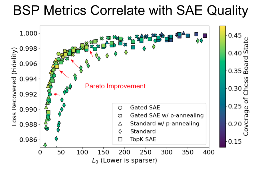
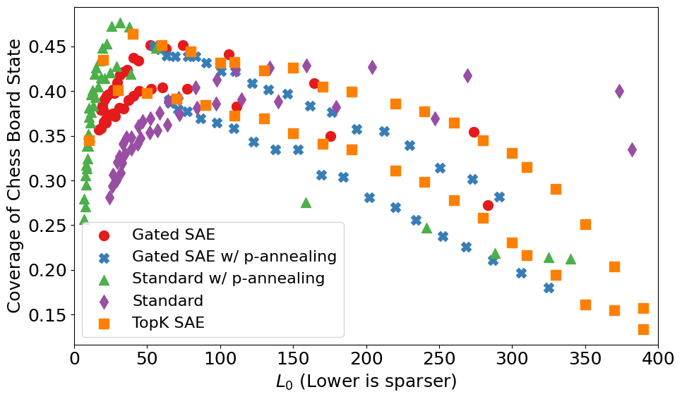
Using our metrics, we can clearly differentiate between training methods and measure progress that is invisible to existing metrics. In this case, we typically see the best performance from SAEs trained with p-annealing, even though their performance is very similar to gated SAEs under proxy metrics. There are also parallel lines within training methods, representing SAEs trained with different expansion factors. These differences are also hiddden within existing metrics.

In this scatter plot, we have L0 on the x-axis and coverage for Chess low-level BSPs on the y axis. Note that TopK was not included in the original paper.

Limitations

The internals of ML models are still poorly understood. Thus, it isn’t clear if our metrics correspond to the “true model ground truth features”, whatever that means. It isn’t clear what the maximum coverage score should be. The field of interpretability is relatively new, and it isn’t clear what the ideal version of these metrics should be. However, I am confident that this an important question to investigate.

We do not capture everything that ChessGPT is doing. Instead, we attempt to measure something that we believe should be present (the state of the board). For high level features like “a fork is present”, it isn’t as clear if ChessGPT actually represents this internally.

In addition, lessons learned from board game models may not transfer to language models. It would be ideal to go straight to language models, but that direction is much less tractable. Thus, an important next step is to investigate if lessons learned here (such as optimal SAE architectures) transfer to language models.

In addition, we find that SAE features fire with high precision for some board states. Although we have qualitatively inspected some features, we haven’t quantitatively investigated how interpretable these features are, or how to quantify interpretability in this case. It would be ideal to integrate interpretability into our analysis.

Implications and Future Work

Interpretability research on restricted domains with a measurable ground truth may enable quantitative comparisons of different approaches that transfer to natural language. In particular, Chess is closer to the complexity of natural language than Othello. The games are generated by real humans instead of being randomly generated, which means there is some sort of theory of mind that can be modeled. We know that ChessGPT already estimates the skill level of players involved. In Chess, tokens are characters, and the model has to combine multiple characters in a semantic unit. In OthelloGPT, a single token represents a single square. In addition, Chess has some concepts at different levels of sparsity, such as check (which is common) and en passant (which is rare).

In general, understanding a model is much more tractable when there is an underlying measurable ground truth. We may be able to use ChessGPT to understand topics analogous to natural language, such as how ChessGPT combines multiple characters into a single semantic unit of a piece being moved. However, it will be important to check if lessons learned here transfer to natural language.

If interested in discussion or collaboration, feel free to contact me via email. I am currently interested in developing evaluations for SAEs trained on language models and doing further reverse-engineering of board game models.

On a personal note, I am currently open to job opportunities. If you found this post interesting and think I could be a good fit for your team, feel free to reach out via email or LinkedIn.

Appendix

Implementation details

For the game of Othello, we classify the board as (Mine, Yours, Empty), rather than (Black, White, Empty), following earlier Chess and Othello work. In Chess, we measure the board state at the location of every “.” in the PGN string, where it is White’s turn to move. Some characters in the PGN string contain little board state information as measured by linear probes, and there is not a clear ground truth board state part way through a move (e.g. the “f” in “Nf3”). We ignore the blank squares when measuring coverage and board reconstruction.

When measuring chess piece locations, we do not measure pieces on their initial starting location, as this correlates with position in the PGN string. An SAE trained on residual stream activations after the first layer of the chess model (which contains very little board state information as measured by linear probes) obtains a board reconstruction F1-score of 0.01 in this setting. If we also measure pieces on their initial starting location, the layer 1 SAE’s F1-score increases to 0.52, as the board can be mostly reconstructed in early game positions purely from the token’s location in the PGN string. Masking the initial board state and blank squares decreases the F1-score of the linear probe from 0.99 to 0.98.

Our SAEs were trained on the residual stream after each layer for 300 million tokens.

Per Layer Performance

We compared SAEs and MLP activations on the tasks of reconstructing all the Chess board, Othello board, and the locations of all valid Othello moves. We selected a high-performing SAE on layer 6, and then used that architecture and hyperparameter selection for training on all other layers. The hyperparameters are probably not optimal for other layers. Most SAEs looked reasonable using proxy metrics, but the layer 3 Chess SAE had less than 100 alive features, leading to very poor performance on our metrics.

It’s notable that the trend of board state information per layer matches across linear probes, SAEs, and MLP activations in both Chess and Othello, indicating that this approach is probably finding something real.

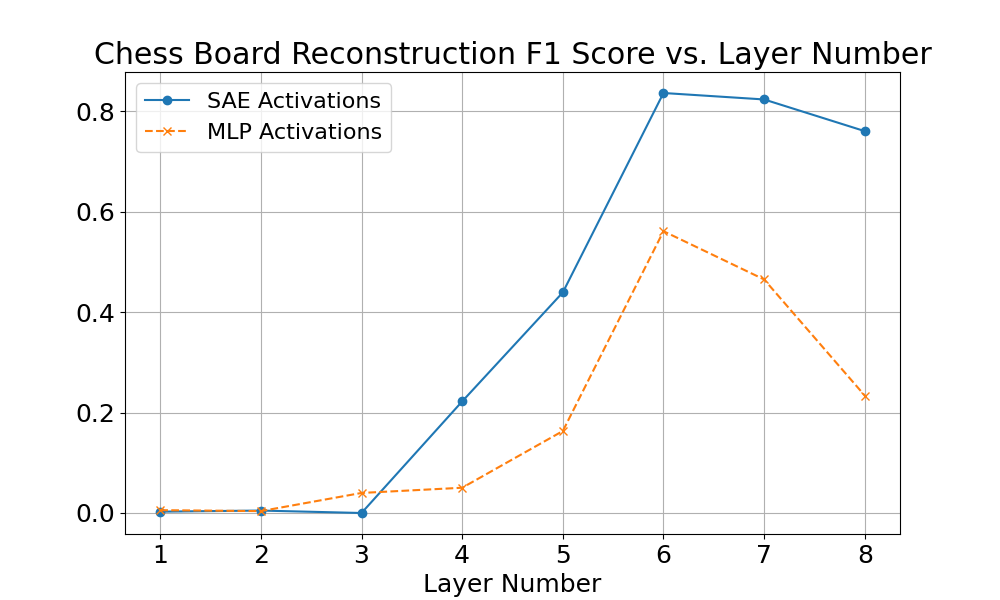
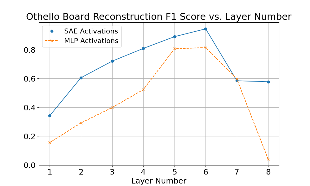
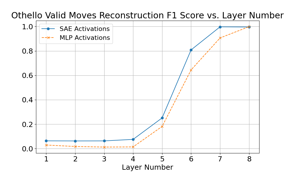
1. It is natural to wonder if it’s a safe assumption that we should be able to recover the board state from a ChessGPT or OthelloGPT model. I have three arguments:

   1. Using linear probes on ChessGPT and OthelloGPT, we can recover over 99% of the board state.

   2. Linear probes are trained with supervision, and may have a correlational, rather than causal relationship with model internals. However, linear probe derived vectors can be used for accurate causal interventions.

   3. There are 10^58 possible Othello games and more possible games of Chess than atoms in the universe. ChessGPT has a legal move rate of 99.8%, and OthelloGPT has a legal move rate of 99.99%. It’s plausible that it’s only possible to achieve this legal move rate by tracking the state of the board.

   I don’t have strong guarantees that ChessGPT and OthelloGPT actually track board state, but it seems like a reasonable assumption. ↩

2. Note that we do not measure pieces on the initial starting position. See Implementation Details in the Appendix. ↩

3. The 20% threshold represents a real valued activation over 20% of its recorded maximum activation. If the maximum activation was 10.0, it was include any value over 2.0. ↩